Editor's Note: As organizations increasingly adopt hybrid work models, the challenge of maintaining team cohesion and culture intensifies. This shift not only redefines collaboration but also raises questions about employee engagement and retention. How can leaders effectively foster a sense of belonging in a dispersed workforce, ensuring that remote employees feel just as valued and connected as their in-office counterparts? Addressing this will be crucial for long-term organizational success.

Building a Llama-Style MoE Language Model From Scratch, Part 1: Architecture and Components

As Large Language Models (LLMs) evolve, the Mixture of Experts (MoE) architecture has become a key innovation for building powerful and efficient models like Llama 3. By combining sparsely activated expert networks with a sophisticated router, an MoE language model expands its capacity while reducing computational costs during inference. But how does a Llama-style MoE architecture work? In this PyTorch tutorial series, we will build a complete MoE model from scratch. This journey covers everything from data preparation and model architecture to the final training loop and inference.

This first installment establishes the conceptual foundation. We will begin with the high-level architecture to build an intuition for the MoE design philosophy. We will then detail the implementation of its core modules—including Multi-Head Attention, RMSNorm, RoPE, and the MoE layer itself—to lay the groundwork for the complete training and inference workflows to come.

Understanding the Llama MoE Architecture

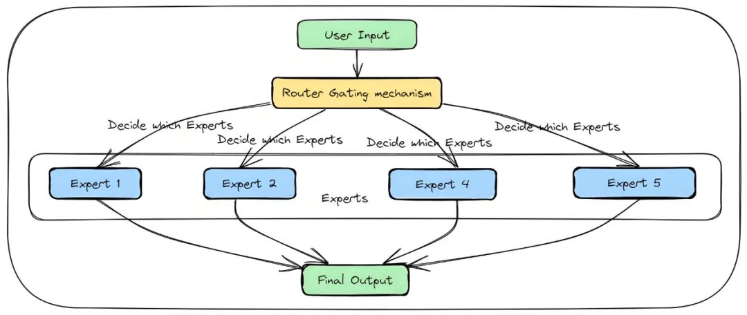
To grasp the Llama MoE architecture, it helps to think of it as a brilliant project manager leading a team of specialized consultants. When faced with a complex problem, this manager doesn't burden every consultant with the entire task. Instead, they intelligently assign pieces of the problem to the most qualified experts, ensuring efficient and effective collaboration.

How MoE Experts Work

Each "expert" is a small, independent neural network, typically a Feed-Forward Network (FFN). While they share the same structure, they have their own unique parameters. This allows each one to develop a specialty—like processing different semantic patterns or grammatical structures—just like a team of human experts.

The Role of the MoE Router

The "router" acts as the dispatcher. For every piece of incoming data (like a word or token), the router analyzes it and intelligently selects a small subset of the most relevant experts to handle the task. The remaining experts stay dormant for that computation cycle.

This "sparse activation" is the critical mechanism behind the Mixture of Experts model. The model can contain a massive number of parameters (experts), giving it vast knowledge, but only a fraction of them are used for any given input, making it incredibly efficient.

Let's walk through a simple example. Consider the sentence: "The dog sat." The model first tokenizes it into "The", "dog", and "sat". We'll focus on the token "dog," which is converted into a vector and fed into an MoE layer.

The router analyzes this vector to decide which experts are best suited to process it. Let's say the model has eight experts (E1-E8), but the router is configured to select the top two.

The vector for "dog" is then passed only to these two selected experts, which produce their respective outputs. These outputs are then combined using a weighted sum (the weights are also determined by the router), and the final result is passed to the next layer. The other six experts remain inactive, saving precious computational resources.

The MoE Language Model Data Pipeline

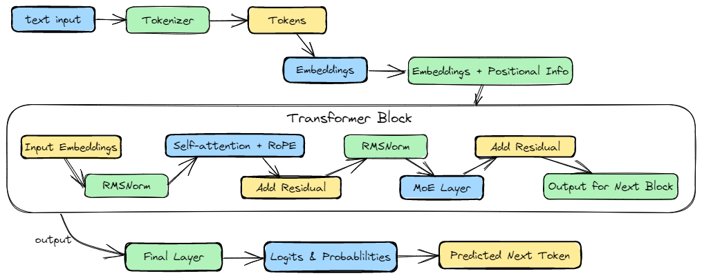
Now let's zoom out and look at the entire data pipeline for our Llama-style MoE model:

1. Tokenizer: The input text is first broken down into a sequence of numerical Token IDs.
2. Embedding Layer: Each Token ID is converted into a dense vector (an embedding). This layer also incorporates positional information, which we'll add using RoPE within the attention mechanism.
3. Transformer Blocks: These vectors then flow through a stack of Transformer blocks. Each block contains two main sub-layers:
   • A Multi-Head Attention mechanism.
   • A Mixture of Experts (MoE) layer (which replaces the traditional FFN).
4. Output Layer: Finally, the processed vectors from the last Transformer block are fed into an output layer. This layer generates "logits"—raw scores for every possible next token in the vocabulary. These scores are then converted into a probability distribution, allowing the model to make its final prediction.

Now that we have a solid high-level understanding, let's begin building these components step by step.

Step 1: Preparing the Training Corpus for our MoE Model

The foundation of any powerful language model is data. Production-grade models like Llama are trained on web-scale corpora containing trillions of tokens.

For our tutorial, however, we'll take a different approach. To keep things manageable and focus on the mechanics, we'll use a tiny, custom corpus. This lets us see exactly how the model processes data at every stage without getting bogged down by massive datasets.

Step 2: Building a Character-Level Tokenizer in PyTorch

Before our model can learn, we need to translate human language into a numerical format it can understand. This process is called tokenization. We'll start with the most fundamental approach: character-level tokenization.

The process is straightforward:

1. Build Vocabulary: We'll scan our corpus and identify every unique character to create our vocabulary.
2. Create Mappings: We'll then create two dictionaries: char_to_int to map each character to a unique integer ID, and int_to_char for the reverse lookup.

Next, we'll use our char_to_int map to encode the entire raw corpus (corpus_raw) into a sequence of integer IDs. This numerical representation is what the model will actually train on. For efficiency, we'll store this sequence as a PyTorch tensor.

We've successfully converted a 594-character text into a PyTorch tensor of shape torch.Size([594]). Each number in this tensor is an ID corresponding to a character, ready to be processed on our target device (e.g., 'cuda').

Step 3: Creating Training Data with a Sliding Window

At its core, a language model is a prediction machine. Its goal is simple: given a sequence of tokens, predict the very next one. To teach it this skill, we need to structure our data into input-target pairs.

We'll use a classic and effective technique: the sliding window. We'll slide a window of a fixed size (block_size) across our corpus, creating a multitude of training examples. For each window, the input (x) will be the first block_size characters, and the target (y) will be the same sequence, shifted one position to the right.

In other words, when the model sees the input context from x[0] to x[t], its job is to predict y[t] as the next character.

This method allows us to extract every possible overlapping segment from the corpus, generating a rich set of training samples that help the model learn linguistic patterns and context.

Success! We've extracted 529 input-target sequence pairs, each 64 characters long. These samples are now ready for training. While train_x and train_y are currently on the CPU, we'll move them to the GPU in batches during the training loop to maximize performance.

Step 4: Implementing a Mini-Batch Data Loader

Feeding an entire dataset into a model at once is computationally infeasible due to memory constraints. This is where mini-batch training is essential.

Instead of training on all the data simultaneously, we'll process it in small, manageable chunks, or "batches." In each training step, we'll randomly select a batch of samples, feed them to the model, and update its parameters.

Here’s how we'll implement it:

1. Generate Random Indices: Create a tensor of batch_size random integers, where each integer is an index into our training set.
2. Slice the Data: Use these random indices to pull the corresponding input and target sequences from train_x and train_y.
3. Move to Device: Transfer the selected batch of data to the active computing device (like a GPU) for processing.

With this function, we can now draw a random batch of 16 samples in each training iteration, providing an efficient stream of data to our model.

Step 5: Defining Hyperparameters for the MoE Language Model

Now we define the blueprint for our model by setting its hyperparameters. These serve as the configurable parameters that control the model's architecture, training behavior, and resource footprint.

Our configuration will be a miniature version of a Llama-style architecture, complete with an MoE layer. Here are the key settings:

• vocab_size: 65 (The number of unique characters in our vocabulary)
• d_model: 128 (The dimensionality of our model's embeddings and hidden states)
• block_size: 64 (The context length or sequence length for each training sample)
• n_heads: 4 (The number of heads in our Multi-Head Attention mechanism)
• n_layers: 4 (The number of Transformer blocks to stack)
• dropout: 0.1 (The dropout rate for regularization)
• n_experts: 8 (The total number of experts in each MoE layer)
• top_k_experts: 2 (The number of experts to activate for each token)

These hyperparameters are a starting point. In a real-world scenario, you'd tune them based on your specific hardware, dataset, and performance goals.

Step 6: Building the Core MoE Model Components

With our data pipeline and hyperparameters defined, we can now initialize the weights for each core component of our MoE language model.

Component 1: The Token Embedding Layer

Every journey begins with a single step, and for our model, that step is the Embedding Layer. This is the model's front door. Its job is to convert each numerical token ID into a dense, high-dimensional vector of size d_model.

The analogy of a "lookup table" is perfect here. Each unique token ID in our vocabulary is mapped to its own dense vector. During training, the model learns to pack semantic meaning into these vectors.

• Input shape: (batch_size, sequence_length)
• Output shape: (batch_size, sequence_length, d_model)

We've successfully created the nn.Embedding layer. With this in place, our model can now transform discrete token IDs into meaningful vector representations, which will be processed by the subsequent Transformer blocks.

Component 2: Implementing Rotary Position Embedding (RoPE)

A standard Transformer architecture is permutation-invariant, meaning it processes input without inherent knowledge of word order. To resolve this, we must inject positional information. Unlike traditional positional encodings, modern architectures like Llama employ a more dynamic solution: Rotary Position Embedding (RoPE).

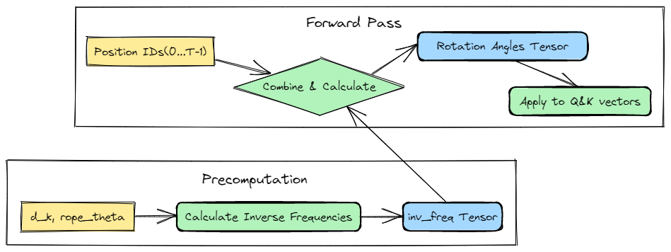
Instead of adding positional data, RoPE integrates it by rotating the query (Q) and key (K) vectors within the attention mechanism. The angle of rotation is a direct function of the token's absolute position in the sequence, elegantly weaving sequential context into the self-attention calculation itself.

To apply these rotations efficiently during the forward pass, we pre-compute a frequency tensor that will be used to calculate the precise rotation angles for each token based on its position:

These inv_freq values are constants that will be used during the forward pass to calculate the precise rotation needed for each token based on its position in the sequence.

Component 3: Using RMSNorm for Model Stability

Training deep neural networks can be an unstable process. Normalization layers act as guardrails to maintain stability. While LayerNorm is common, Llama opts for a leaner, more efficient alternative: RMSNorm (Root Mean Square Normalization).

The key difference? RMSNorm simplifies the process by skipping the mean-centering step. It only scales the input by its root mean square, then applies a learnable gain parameter (gamma). This small change yields significant performance gains in the Transformer architecture.

In our model, an RMSNorm layer precedes each Attention and MoE module, with a final one applied just before the output layer. Here, we'll initialize the learnable gamma weights for all these layers.

For a model with n_layers Transformer blocks, we need gamma weights for:

1. Attention Norms: One for the input of each attention layer.
2. FFN/MoE Norms: One for the input of each MoE layer.
3. Final Output Norm: A single norm before the final projection.

Component 4: The Multi-Head Attention (MHA) Mechanism

The engine of any Transformer is the self-attention mechanism. We'll implement the widely-used Multi-Head Attention (MHA) variant. This allows the model to focus on different parts of the input sequence simultaneously, capturing a richer set of relationships.

For each Transformer layer, we need two key sets of linear projections:

• QKV Projections: A single linear layer that transforms the input vector into three distinct representations: the Query (Q), Key (K), and Value (V).
• Output Projection: After the attention scores are calculated and applied to the Value vectors, this layer combines the results from all attention heads and projects them back to the model's original dimension (d_model).

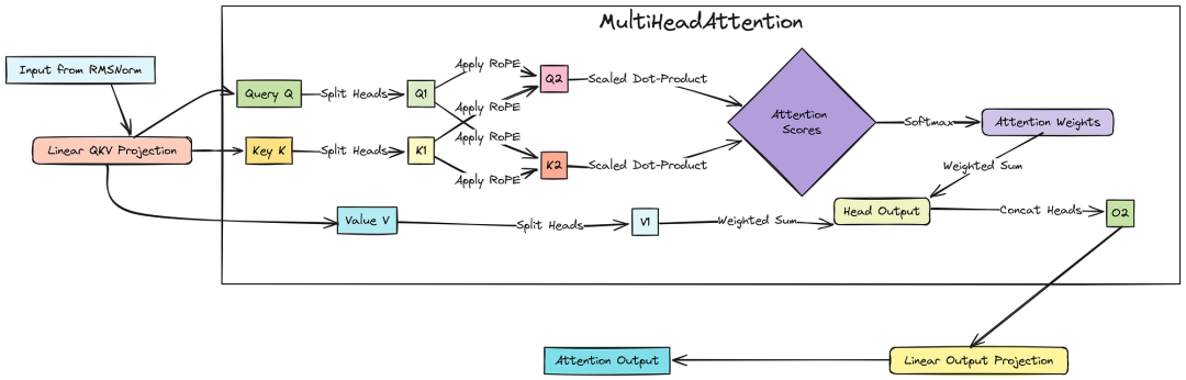
All weights are stored in lists (mha_qkv_linears and mha_output_linears), allowing us to easily access the correct layer's weights during the forward pass.

Component 5: The Mixture of Experts (MoE) Layer

Here, we replace the standard Feed-Forward Network (FFN) with the more powerful Mixture of Experts (MoE) layer. In a traditional Transformer, the FFN is a significant contributor to the model's parameter count. With MoE, we substitute this single, dense FFN with a collection of smaller, specialized 'expert' networks.

The key innovation is sparse activation: for any given token, only a small subset of experts is activated. This allows the model's total parameter count—and thus its knowledge capacity—to increase dramatically without a proportional rise in computational cost.

The essential components for each MoE layer are:

• Router (or Gate): A linear layer that calculates affinity scores to determine which experts are most relevant for the current token.
• Experts: A set of parallel FFNs, each with independent weights, allowing for specialization. In modern designs, each expert is often an FFN with a SwiGLU activation, which consists of three weight matrices: w1 and w3 for the gated linear unit, and w2 for the down-projection.

We will initialize the weights for the router and all experts for each layer in the model:

1. Router Weights: moe_gate_linears
2. Expert Weights: moe_experts_w1, moe_experts_w2, moe_experts_w3

Component 6: The Final Output Layer (Language Model Head)

After the final Transformer layer has processed the input, we have a set of highly contextualized vectors. The last step is to translate these vectors back into token predictions. This is the job of the output layer, often called the "un-embedding" or "language model head."

After a final RMSNorm, a linear projection layer maps the d_model-dimensional vector into a much larger vector with a size equal to our vocabulary (vocab_size).

Each element in this output vector is a logit—a raw, unnormalized score for a potential next token. A softmax function then converts these logits into probabilities, and the model predicts the token with the highest probability.

Component 7: Enforcing Autoregressive Behavior with a Causal Mask

Language models like the one we're building are autoregressive, meaning they generate text one token at a time. This imposes a fundamental rule: when predicting the next token, the model can only attend to tokens that came before it. It cannot see into the future.

This rule is enforced by the Causal Mask. During the self-attention calculation, we apply a mask that conceals all future tokens from the current position. This mask is a lower-triangular matrix where:

• Values on and below the diagonal are 1 (or True), allowing attention.
• Values above the diagonal are 0 (or False), preventing attention.

This ensures that the prediction for token t can only depend on tokens 0 through t-1, preserving the model's autoregressive property.

Summary and Next Steps

In this first installment, we have laid the essential groundwork for our Llama-style MoE model. We explored the theory behind the Mixture of Experts architecture and detailed the initialization of every core component—from data preparation and tokenization to the specifics of RoPE, RMSNorm, Multi-Head Attention, and the MoE layer itself.

Stay tuned for the next article, where we will assemble these building blocks into a complete, end-to-end model. We will implement the training loop, define our loss function, and watch our model generate its first lines of text. By the end of the series, you will have a fully functional MoE-based language model running on your machine.

Key Takeaways

• Understand the Mixture of Experts (MoE) architecture for efficient language model development.
• Learn to implement RMSNorm and RoPE in your MoE model design.
• Follow a step-by-step PyTorch tutorial to build a Llama-style MoE model.