Understanding Multi-head Latent Attention (MLA)
In modern large language models, vanilla Attention is becoming a rarity. For tasks ranging from KV cache optimization to implementing novel attention variants, Multi-head Latent Attention (MLA) has emerged as a new fundamental building block for efficient LLM inference.
Despite its widespread adoption, a deep, intuitive understanding of how Multi-head Latent Attention works remains elusive. Many engineers grasp high-level concepts—like matrix absorption or the distinction between prefill and decode modes—but the specific operational details are often unclear. How precisely do the prefill and decode computations differ? How are parameter matrices rearranged to optimize GPU performance? This ambiguity can lead to oversimplifications, such as dismissing MLA as a mere 'space-for-time tradeoff.'
The challenge often stems from explanations grounded in pure matrix algebra, which can obscure the multi-dimensional nature of deep learning tensors. For practitioners accustomed to frameworks like PyTorch, thinking in terms of tensor shapes provides a more direct path to clarity.
This article aims to bridge that gap. Using flowcharts that map the MLA computation process to PyTorch-style tensor shapes, we will build an intuitive, visual understanding of its inner workings. The goal is to provide a mental model so clear that a single glance at a diagram is all that's needed for a complete refresh.
How MLA Works: Prefill vs. Decode Phases
Multi-head Latent Attention uses a dual-path architecture, with distinct computational graphs for the initial processing (prefill) and subsequent token generation (decode).
The Prefill Phase: Building the KV Cache with MHA
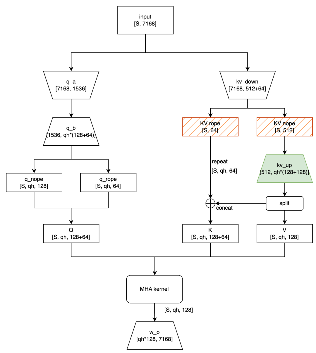
In this flowchart, rectangular boxes represent intermediate activations, while trapezoids are the model's learnable parameters. The numbers denote the tensor shapes. For our example, let's say the sequence length is S and the number of query heads is qh. To keep things clean, we'll stick to the dimensions from the original paper and omit operations like LayerNorm.
The core of the MLA prefill phase is a two-step projection process: a down-projection followed by an up-projection. The input is multiplied first by q_a and then q_b (for the query), or by kv_down and kv_up (for the key and value). The red diagonal lines highlight a key step for KV cache optimization: the down-projected KV tensors—both with RoPE applied and without (the 'base' tensor)—are saved to the KV cache for the upcoming decode phase.
A clever trick here is that while the Q tensor is multi-headed, the corresponding K tensor is single-headed. This single-headed K is then replicated across all heads and concatenated with the up-projected tensor to form the final multi-headed K. This is a subtle but powerful technique for LLM optimization.
At this stage, the up-projected Q, K, and V are all multi-headed. This means they are perfectly formatted to be fed into a standard Multi-Head Attention (MHA) operator, like the highly optimized FlashAttention kernel.
The Decode Phase: Efficient Generation with MQA
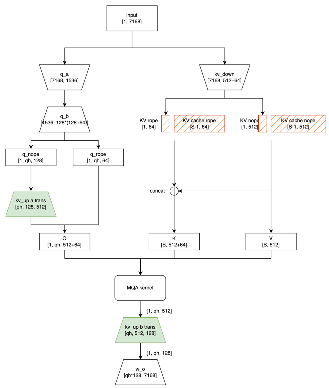
The decode phase is where the optimization of Multi-head Latent Attention truly shines. Here, we process one token at a time. Assuming our KV cache already contains S-1 tokens, the key tensor for the new token is concatenated with this cache, creating a combined key tensor of shape [S, 512].
Notice two new parameter matrices in the diagram: kv_up a trans and kv_up b trans. These aren't new weights; they're derived from the original kv_up matrix through a process called matrix absorption.
The Core Optimization: Matrix Absorption Explained
Matrix absorption is the central optimization that makes the MLA decode phase so efficient. It rearranges the computation to avoid costly operations on the large, cached Key and Value tensors.
How Matrix Absorption Works in MLA
Let's break down how matrix absorption works. In the prefill phase, the base KV tensor (without RoPE) is multiplied by the kv_up matrix:

The @ symbol denotes matrix multiplication. The result is then reshaped and split to form the final K and V tensors.
The magic of matrix absorption comes from the associative property of matrix multiplication. Instead of calculating (A @ B) @ C, we can calculate A @ (B @ C) to get the same result.
In our case, the calculation for attention scores involves a term like (q_base @ kv_up_k_weight). In the decode phase, we can pre-compute the equivalent of kv_up_k_weight to create kv_up a trans. Let's trace the shapes. For a single token and a single head, q_base has a shape of [1, 128]. By re-associating the multiplication, we effectively multiply q_base by the transpose of the weight matrix, which is [128, 512].
So, for each head, we perform a [1, 128] @ [128, 512] multiplication, yielding a [1, 512] tensor. This is the 'absorption': we've absorbed the up-projection for K directly into the Q-path computation.
From MHA to MQA: A Strategic Shift
After this absorption step, Q is multi-headed, but K remains single-headed. This structure is a perfect fit for a Multi-Query Attention (MQA) operator. It's a specialized form of MQA where the number of KV heads is just one. This design choice is a key motivation behind custom operators like FlashMLA, as it significantly improves GPU performance during decoding.
The same logic applies to kv_up b trans, which is used after the MQA computation to transform the output.
Performance Analysis: MHA vs. MQA in MLA
The dual-path architecture of MLA isn't just a mathematical trick; it's a strategic choice to optimize performance by increasing computational density. The decision of which path to use depends on the workload.
A Dynamic Trade-off for LLM Inference
To understand the trade-offs, let's analyze the computational costs. Let x be the number of new input tokens and y be the length of the existing KV cache.
- Non-Absorbed (MHA) Path: This path performs a large up-projection on the entire Key and Value sequence (
x+ytokens). Its cost is dominated by this step and scales significantly with the total sequence length. - Absorbed (MQA) Path: This path avoids the large KV up-projection. Instead, it performs smaller, re-associated multiplications on the query side (
xtokens). Its cost is more sensitive to the number of new tokens.
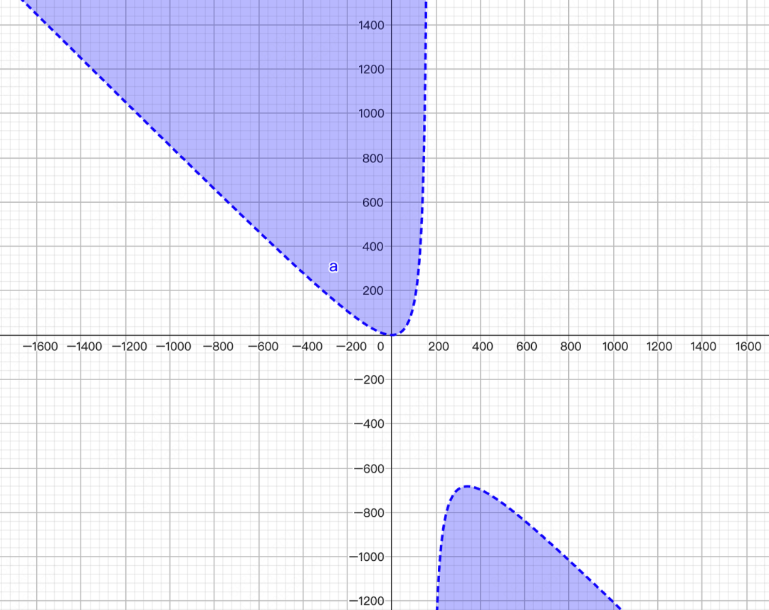
By modeling the floating-point operations, we can establish a hyperbolic decision boundary when plotted against x and y.
Practical Applications: Chunked Prefill & Speculative Decoding
This analysis gives us a dynamic strategy for picking the most efficient kernel in modern LLM inference scenarios like chunked prefill, prefix caching, and speculative decoding, where we might process a batch of new tokens (x > 1) while the KV cache is populated (y > 0).
The key takeaway is this: when x is large (roughly x > 170), the non-absorbed MHA path is actually cheaper, regardless of the cache length y.
This has direct practical implications:
- For chunked prefill, where
xis large (e.g., 2048), you should use the non-absorbed MHA approach. - For speculative decoding, where
xis small, the absorbed MQA path is the clear winner for LLM optimization.
Of course, the non-absorbed path creates large intermediate K and V activation tensors, which can consume significant VRAM. But that is a topic for another time.
Hardware-Aware Design: Why MQA Optimizes GPU Performance
We've established that the absorbed MQA path is ideal for small x, but there's a deeper, hardware-level reason for this design: computational density.
Maximizing Computational Density on GPUs
MQA packs more arithmetic operations into each byte of data read from memory, which is crucial for maximizing GPU performance. In the decode phase, we can fuse the head-by-head attention score calculations into a single, large matrix multiplication: [qh, 576] @ [576, S].
This is where the design meets the hardware. Modern GPUs like NVIDIA's Hopper series use specialized instructions like wgmma that are most efficient when matrix dimensions are large (e.g., the M dimension is at least 64). For a model with qh=128, the M dimension is 128, which perfectly utilizes the wgmma instruction's power. This high computational density helps shift the notoriously memory-bound decode step towards being compute-bound.
In contrast, running the non-absorbed MHA path during decode would involve a batched matrix multiply where the M dimension is just 1, which is horribly inefficient for modern tensor cores.
Solving the Tensor Parallelism Challenge
What about Tensor Parallelism (TP)? If we split the model across 8 GPUs, each GPU might only handle qh = 16 heads, making the M dimension too small. This is where speculative decoding comes to the rescue again. If we're verifying x speculative tokens at once, the Q shape becomes [x, qh, 576]. We can reshape this into a single large matrix multiplication: [x*qh, 576] @ [576, S]. As long as x * qh is a multiple of 64 (e.g., x=4 speculative tokens on a TP=8 setup gives 4 * 16 = 64), we can once again achieve maximum hardware utilization.
Conclusion: Key Takeaways on MLA
We have journeyed deep into the mechanics of Multi-head Latent Attention, moving from high-level architecture to hardware-level optimization. The key takeaways are:
- Dual-Path Architecture: MLA employs two distinct paths—an MHA-based prefill stage and an MQA-based decode stage—which can be clearly understood through visual flowcharts and tensor shapes.
- Dynamic Optimization: The choice between the 'non-absorbed' (MHA) and 'absorbed' (MQA) methods is a dynamic optimization problem, with a clear crossover point based on the number of new input tokens.
- Hardware-Aware Design: The switch to MQA in the decode phase is a deliberate strategy to maximize computational density and fully leverage the matrix multiplication capabilities of modern GPU tensor cores.
This breakdown should demystify Multi-head Latent Attention, providing an intuitive mental model that connects its theoretical underpinnings to its practical performance benefits in LLM optimization.
The views expressed in this article are my own and do not reflect those of my employer.
[1] GTA, GLA: https://arxiv.org/abs/2505.21487