Monitoring PyTorch GPU memory usage during model training can be perplexing. To demystify this, we'll dive into the PyTorch memory snapshot tool, a powerful utility for detailed GPU memory analysis during both training and inference. While other guides cover basic operations, our focus is on interpreting the rich data these snapshots provide. Using mixed-precision training (AMP) as a case study, we will trace how memory is allocated, used, and released. This guide will equip you with the skills to diagnose and solve complex PyTorch memory issues in your own deep learning projects.
Understanding the PyTorch Memory Snapshot Tool
To effectively interpret a PyTorch memory snapshot, you must first understand a core concept: PyTorch's memory caching.
How the PyTorch Caching Allocator Works
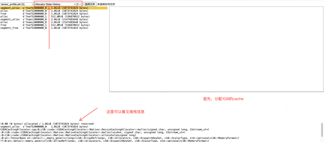
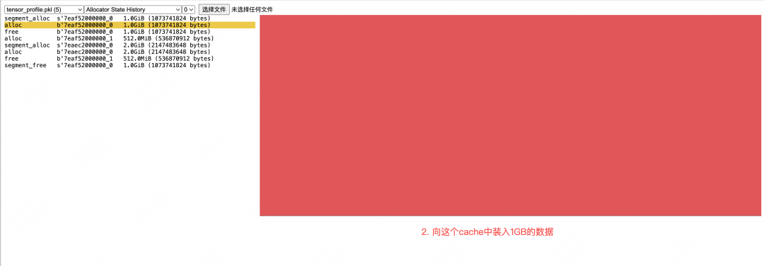
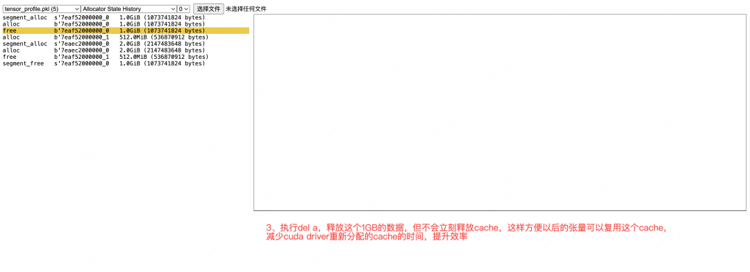
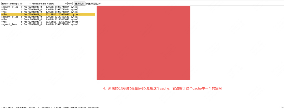
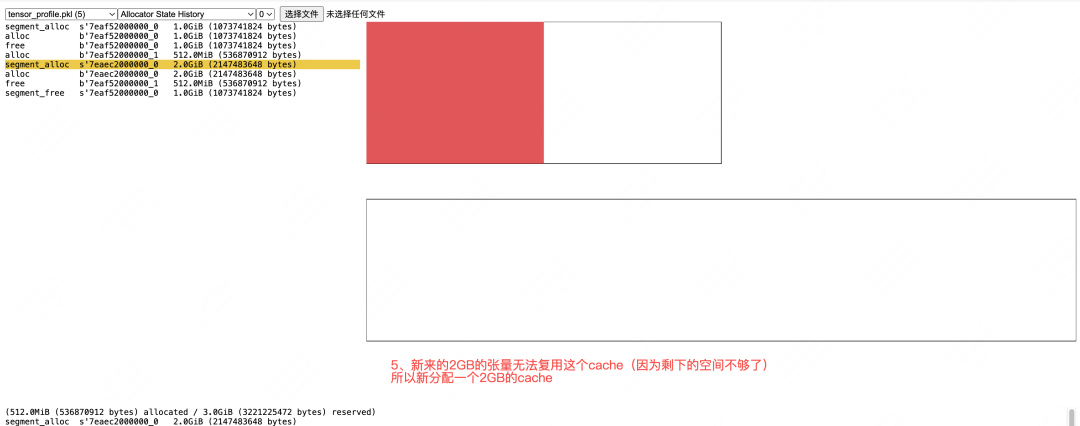
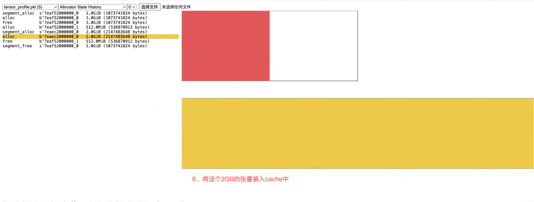
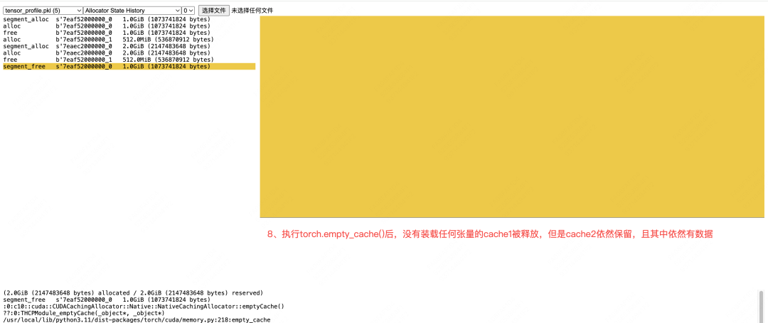
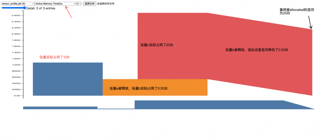
For clarity and accessibility, this analysis prioritizes building intuition. In memory snapshots, you will encounter the term "allocating a cache buffer." This refers to the PyTorch caching allocator's behavior. When a segment of GPU memory is needed, PyTorch requests it from the driver. Once the tensors in that segment are no longer needed, PyTorch does not immediately release the memory back to the GPU. Instead, it retains the empty block in a pool of available memory for future requests. This strategy minimizes the performance overhead of frequent memory allocation calls to the driver. Throughout this article, we will refer to this mechanism as caching.
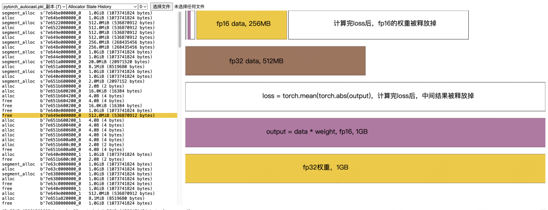
GPU Memory Analysis of the Forward Pass
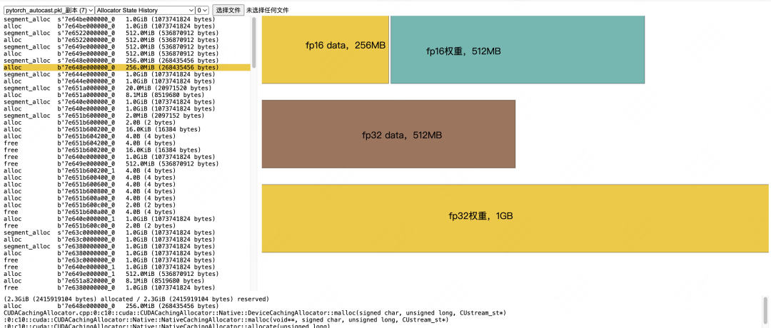
Let's begin our GPU memory analysis by examining the forward pass of a training step. We will trace memory from initial allocation for weights and data to the creation of activations.
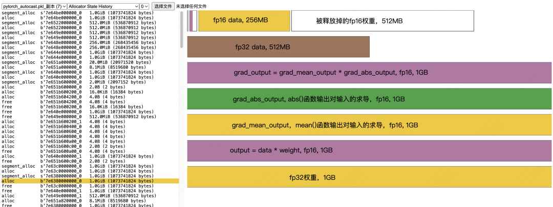
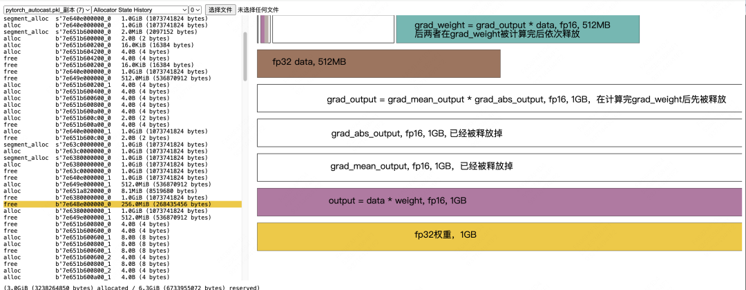
GPU Memory Analysis of the Backward Pass
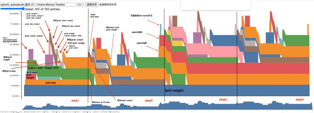
Next, we analyze the backward pass, where the bulk of GPU memory optimization opportunities lie. This phase involves gradient calculation and the subsequent release of memory used by activations from the forward pass.
After walking through the first training step, you likely have questions about the observed PyTorch memory usage. Let's tackle them one by one.
Common PyTorch Memory Questions Answered
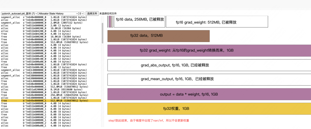
Why are there no weight updates in step 1?
The reason lies in how mixed-precision training handles overflows. The gradients calculated in step 1 contained NaN/Inf values, signaling an overflow. Consequently, the optimizer step, including the weight update, was skipped. The Adam optimizer's momentum buffers—the first and second moment estimates—are initialized lazily. They are only created upon the first successful weight update, which is why they do not appear in the PyTorch memory snapshot until a valid step is completed.
Why isn't memory for output = data * weight freed until step 2?
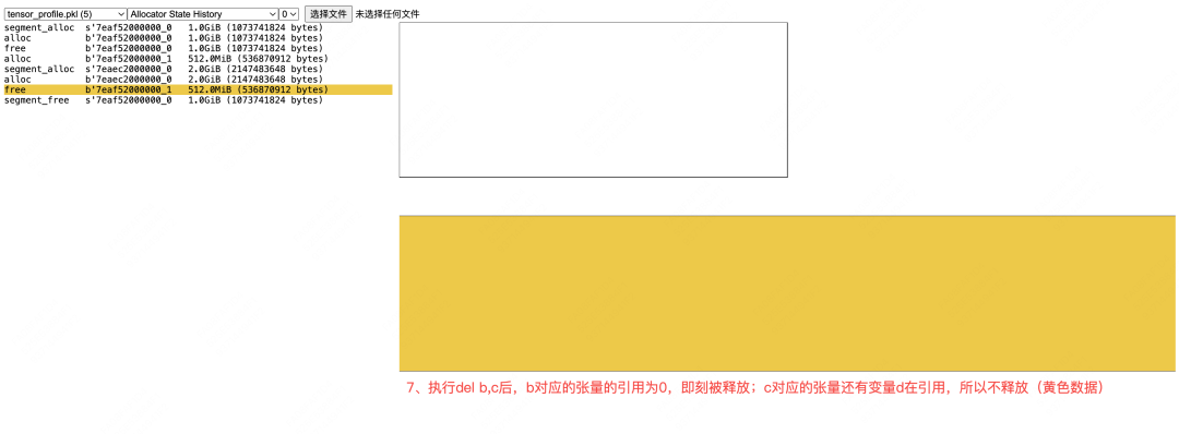
This highlights a common aspect of PyTorch memory management. While the output activation is no longer needed after its gradient is computed, its memory is not immediately freed due to a lingering reference from the training loop. The line output = model(data) creates a Python variable holding a reference to the GPU tensor. This reference prevents deallocation. Only when the line is executed again in the next step is the original reference overwritten, allowing the garbage collector to release the memory.
When is the fp32 grad_weight released?
At the end of step 1, we allocated memory for the fp32 grad_weight. Because the gradients overflowed, it was never used. This stale grad_weight from step 1 is released after the forward pass memory usage of step 2 completes but before the backward pass begins. This timing is a direct consequence of the internal implementation of Automatic Mixed Precision (AMP).
The Active Memory timeline is dense. How can I get more detail?
The detailed annotations in the diagrams are derived by cross-referencing the PyTorch memory snapshot's stack trace with the source code. While the timeline can appear cryptic, this method provides a clear path to deciphering it. By stepping through the stack trace for each allocation and deallocation event, you can pinpoint the exact line of code responsible.
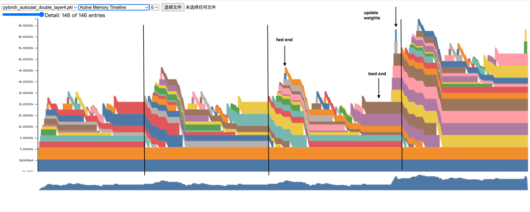
Advanced Memory Analysis: Multi-Layer Models and Distributed Training
With the concepts from our GPU memory analysis covered, this next section should be easier to digest. Here's a direct interpretation of the memory timeline for a two-layer model, where you can clearly see how cached memory blocks are reused.
Loading and Precision Conversion of Data and Weights:
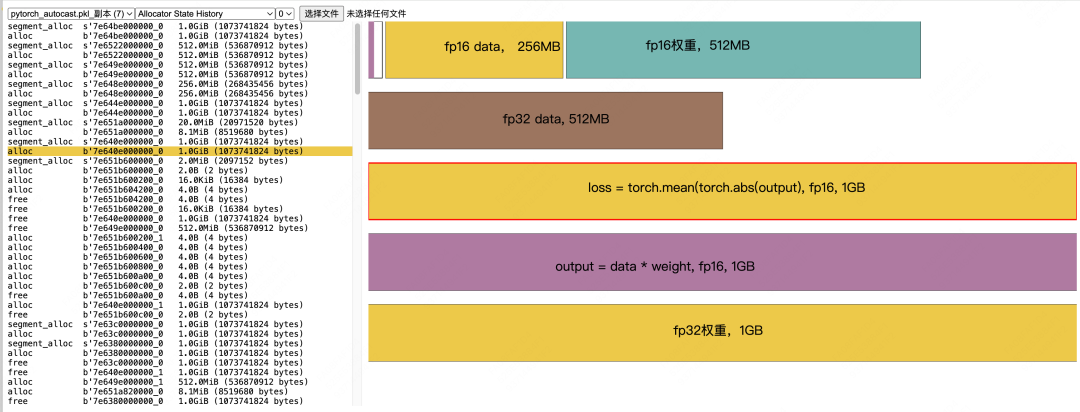
Output and Loss Calculation:
Memory Release After Loss Calculation:
Calculation of grad_output and Subsequent Memory Release:
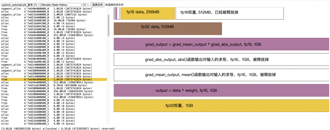
Calculation of fp16 grad_weight and Subsequent Data Release
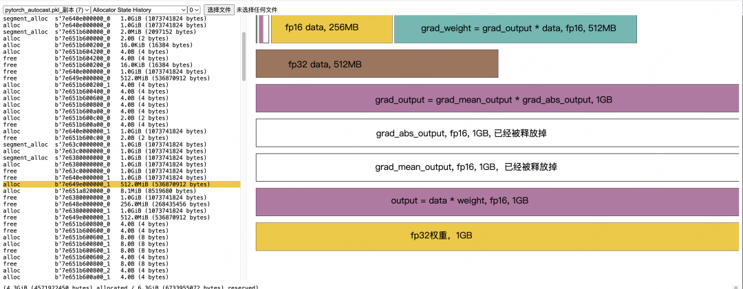
Converting fp16 grad_weight to fp32 grad_weight:
I encourage you to use the stack trace method to map out the remaining events. This is a valuable exercise for understanding the intricacies of the training process, like the precise timing of fp32 gradient generation and activation release.
This same investigative technique scales to complex scenarios like ZeRO-1 distributed training. The snapshot below is from a two-GPU toy example (rank 1).
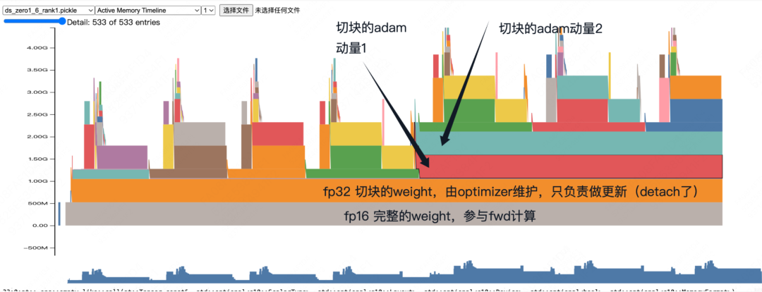
By systematically reviewing the source code using the stack trace, we can outline the entire distributed process. This reveals interesting details, such as how in ZeRO-1, fp16 weights are stored persistently, unlike in standard AMP where they are temporary. We can also spot memory allocations related to distributed communication.
By mastering the art of interpreting a PyTorch memory snapshot, you move from being a passive observer of GPU memory to an active investigator. The ability to cross-reference stack traces with your source code is a fundamental skill that demystifies complex frameworks like AMP and ZeRO, enabling you to write more efficient and robust code.